卷积和循环神经网络中每个时刻只能捕捉相邻位置元素的关系,而作者受到非局部均值滤波去噪算法的启发,设计了一个非局部网络块用来建模任意位置元素的关系,是自注意力应用于视觉任务的扩展,本质也可以看作“加权平均求和”。作者提出的通用的非局部网络块可以灵活地处理图像、序列、视频等多种任务,且可以放在网络的任意位置,在多个视觉任务中均使得模型效果提升。
卷积网络通过卷积核对相邻位置的元素进行建模(局部操作),如果需要建模远距离位置的话需要堆叠多个卷积核;而循环神经网络需要堆叠RNN块,依赖上一时刻的隐状态来预测当前时刻的输出(局部操作),从而对相邻位置的元素进行建模。这两种网络的“局部”操作带来的问题主要有:
- 计算低效,当两个元素的位置很远时,需要堆叠很多操作才能建立两者之间的联系;
- 优化困难;
- 多跳依赖建模(multihop dependency modeling)困难,例如在两个远距离位置来回传递消息非常困难。
而非局部操作的优势体现在:
- 不论距离远近,可以直接对两个位置的元素建模;
- 实验证明,非局部操作高效,且可以使用较少的层实现最佳效果;
- 灵活适应不同的输入尺寸,且与其他操作可以直接组合(“即插即用”)
有趣的是,作者提到这篇非局部网络模块与Transformer中的自注意力模块非常相似,self-attention通过关注所有位置(查询、加权求和)来预测某个位置的输出,而这可以看作非局部均值的一种形式,因此可以将这篇工作看到将机器翻译任务中提出的self-attention扩展到更通用的任务中。
笔者认为这篇非局部神经网络的贡献主要有两点:
- 将自注意力扩展到更加通用的任务中;
- 解释了自注意力有效的关键原因是非局部计算机制,而非QKV的具体计算设计、softmax等。
本文是笔者的个人理解与总结,如果有误欢迎指出交流!
非局部均值滤波
在介绍这篇非局部网络之前,我们先来简单看一下“非局部均值滤波”的思路。(下面我只做一些浅显的介绍,如果读者需要深入了解,可以参考 这篇博客)
传统的图像处理算子受限于算子的大小,每次计算只能关注相邻位置的信息,例如3*3的均值滤波计算时只能考虑附近的9个元素:
\[\begin{equation} \left[ \begin{array}{ccc} 1/3 & 1/3 & 1/3 \\ 1/3 & 1/3 & 1/3 \\ 1/3 & 1/3 & 1/3 \end{array} \right] \end{equation}\]而当图像中距离较远的像素存在强相关性时,普通的算子难以建模这种关系,因此出现了“非局部均值滤波”,其核心思想是:当前像素的估计值由图像中与它具有相似邻域结构的像素加权平均得到,可以简单理解为当前像素的估计值是与图像中所有像素的加权平均。(其实到这里稍微思考一下就会觉得这也是Attention的主要思想,key和query计算的是注意力权重,再与value进行计算也就是加权求和)
基本原理
下面来定义一下网络中非局部操作的计算,当前计算元素的索引为$i$,$j$代表所有位置的索引,$x$为输入数据(可以是图像、序列、视频及其特征),$y$是输出(与输出同尺寸)。
\[\begin{equation} y_{i}=\frac{1}{C(x)}\sum_{\forall{j}}f(x_{i},x_{j})g(x_{j}) \end{equation}\]函数$f$计算两个$x$的关系,得到权重(标量);函数$g$用于提取$j$位置元素的表示。(这里也可以类比Attention机制,$f(x_{i},x_{j})$相当于 key和 query计算,而$g(x_{j})$相当于 value)另外为了数值稳定性,在求和之后使用$C(x)=\sum_{\forall{j}}f(x_{i},x_{j})$约束输出。计算公式中可以看到,预测当前位置时,会和所有位置的元素进行计算,那么就实现了“直接建模任意位置元素的关系”。
而需要注意的是非局部操作不是全连接层$f_{c}$,作者做了几点说明:
- 非局部操作中$f$用于计算不同位置元素的关系,而$f_{c}$中包括可学习的权重;
- $f$允许任意尺寸的输入,而$f_{c}$的输入尺寸固定;
- 非局部神经网络块可以“即插即用”,而$f$只能放在网络输出。
下面我们针对公式2中函数$f$和$g$的设计进行讨论,探究不同的函数对模型效果的影响。
函数构件的设计
首先作者给出了结论:非局部网络对函数的选择并不敏感,使得模型效果提升的关键原因是非局部的机制。
为了简化起见,对于函数$g$,作者设计$g(x_{j})=W_{g}x_{j}$,其中$W_{g}$是可学习的参数,可使用线性层或者卷积操作实现。而对于函数$f$,可使用非局部均值滤波中的高斯函数:
\[\begin{equation} f(x_{i}, x_{j}) = e^{x_{i}^{T}x_{j}} \end{equation}\]其中$x_{i}^{T}x_{j}$为点积相似度(是不是很像点积注意力)。和Transformer中选择缩放点积注意力的原因相似,作者也提到由于矩阵计算效率很高因此使用点积相似度计算。
在点积相似度的基础上,引入可学习的参数,那么可以表示为:
\[\begin{equation} f(x_{i}, x_{j}) = e^{\theta(x_{i})^{T}\phi(x_{j})} \end{equation}\]其中$\theta(x_{i})=W_{\theta}x_{i}$,$\phi(x_{j})=W_{\phi}x_{j}$,相当于在计算之前经过了线性层(很像Transformer的多头自注意力模块中,QKV首先经过了线性层处理)
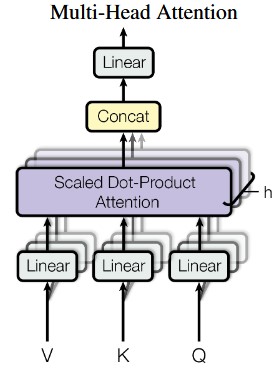
到这里可以看到非局部网络块中的很多内容与自注意力模块相似,因此可以将自注意力模块看作一种特殊的非局部网络块,写作:
\[\begin{equation} y =softmax(x^{T} W_{\theta}^{T} W_{\phi}^{T}x)g(x) \end{equation}\]这样就可以与自注意力模块统一起来,并且将NLP领域的任务自然地过渡到视觉等通过用任务中。
接着作者为了验证影响模型效果的关键因素是非局部计算而不是自注意力函数的设计,设计了两个不同的函数:
-
点积相似性:
\[\begin{equation} f(x_{i}, x_{j}) = \theta(x_{i})^{T}\phi(x_{j}) \end{equation}\] -
concation(拼接后经过线性激活层)
\[\begin{equation} f(x_{i}, x_{j}) = ReLU(w_{f}^{T}[\theta(x_{i}), \phi(x_{j})]) \end{equation}\]
实验表明影响非局部神经网络的关键因素是“非局部计算操作”,其中函数选择的影响很小。
非局部块
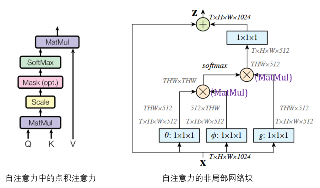
上面讨论非局部计算公式之后,我们来讨论一下非局部块如何设计。上面非局部计算得到位置$i$处的结果$y_i$,非局部块在此基础上添加了可学习的权重$W_z$和残差连接:
\[\begin{equation} z_{i} = W_{z}y_i+x_i \end{equation}\]实现中,作者将非局部计算中的可学习的权重$W_g, W_\theta, W_\phi$的通道均设置为输入通道的一半,而$W_z$通道与输入一致。另外考虑到非局部函数中每次计算时需要与所有元素进行计算,为了加速这一过程,设计了一个简化的版本——子采样版本(其中的$\hat{x}$是$x$的采样版本,例如池化):
\[\begin{equation} y_{i} = \frac{1}{C(\hat{x})}f(x_{i}, \hat{x}_{j})g(\hat{x}_{j}) \end{equation}\]非局部网络块的一个实现见下图,可以看到输入输出尺寸相同,因此是一种“即插即用”的模块。
何时放置非局部块
作为即插即用的模块,其可以放在网络的任一位置,但不同位置处网络效果有较大的差异,作者的实验中看到放在网络的较高层可以获得更好的性能。
此外作者关于计算量、网络深度等部分的讨论在此略去,感兴趣的读者可以自行阅读。
代码实现
笔者选择了github上pytorch版本的实现,首先看一下非局部模块的实现:
class NLBlockND(nn.Module):
    def __init__(self, in_channels, inter_channels=None, mode='embedded',
                 dimension=3, bn_layer=True):
        """提供了4种非局部的计算,但是没有使用论文中提到的sub-sample的trick优化
        args:
            in_channels: original channel size (1024 in the paper)
            inter_channels: channel size inside the block if not specifed reduced to half (512 in the paper)
            mode: supports Gaussian, Embedded Gaussian, Dot Product, and Concatenation,可选的4种非局部计算
            dimension: can be 1 (temporal), 2 (spatial), 3 (spatiotemporal)
            bn_layer: whether to add batch norm
	另:为了方便代码的说明,笔者沿用了自注意力的Q、K、V的名字,读者只需要与非局部块的部分对应起来即可
        """
        super(NLBlockND, self).__init__()

        assert dimension in [1, 2, 3]

        if mode not in ['gaussian', 'embedded', 'dot', 'concatenate']:
            raise ValueError('`mode` must be one of `gaussian`, `embedded`, `dot` or `concatenate`')

        self.mode = mode
        self.dimension = dimension

        self.in_channels = in_channels
        self.inter_channels = inter_channels

        # the channel size is reduced to half inside the block
	# 对应论文中的通道数减半
        if self.inter_channels is None:
            self.inter_channels = in_channels // 2
            if self.inter_channels == 0:
                self.inter_channels = 1

        # assign appropriate convolutional, max pool, and batch norm layers for different dimensions
        if dimension == 3:
            conv_nd = nn.Conv3d
            max_pool_layer = nn.MaxPool3d(kernel_size=(1, 2, 2))
            bn = nn.BatchNorm3d
        elif dimension == 2:
            conv_nd = nn.Conv2d
            max_pool_layer = nn.MaxPool2d(kernel_size=(2, 2))
            bn = nn.BatchNorm2d
        else:
            conv_nd = nn.Conv1d
            max_pool_layer = nn.MaxPool1d(kernel_size=(2))
            bn = nn.BatchNorm1d

        # function g in the paper which goes through conv. with kernel size 1
	# g函数是为了计算“V”,通道数和输入通道数一致
        self.g = conv_nd(in_channels=self.in_channels, out_channels=self.inter_channels, kernel_size=1)

        # add BatchNorm layer after the last conv layer
	# 这里对应 z = W_z * y + x,也就是最后一层
        if bn_layer:
            self.W_z = nn.Sequential(
                    conv_nd(in_channels=self.inter_channels, out_channels=self.in_channels, kernel_size=1),
                    bn(self.in_channels)
                )
            # from section 4.1 of the paper, initializing params of BN ensures that the initial state of non-local block is identity mapping
            nn.init.constant_(self.W_z[1].weight, 0)
            nn.init.constant_(self.W_z[1].bias, 0)
        else:
            self.W_z = conv_nd(in_channels=self.inter_channels, out_channels=self.in_channels, kernel_size=1)

            # from section 3.3 of the paper by initializing Wz to 0, this block can be inserted to any existing architecture
            nn.init.constant_(self.W_z.weight, 0)
            nn.init.constant_(self.W_z.bias, 0)

        # define theta and phi for all operations except gaussian
        if self.mode == "embedded" or self.mode == "dot" or self.mode == "concatenate":
            self.theta = conv_nd(in_channels=self.in_channels, out_channels=self.inter_channels, kernel_size=1)
            self.phi = conv_nd(in_channels=self.in_channels, out_channels=self.inter_channels, kernel_size=1)

        if self.mode == "concatenate":
            self.W_f = nn.Sequential(
                    nn.Conv2d(in_channels=self.inter_channels * 2, out_channels=1, kernel_size=1),
                    nn.ReLU()
                )

    def forward(self, x):
        """
        args
            x: (N, C, T, H, W) for dimension=3; (N, C, H, W) for dimension 2; (N, C, T) for dimension 1
        """

        batch_size = x.size(0)

        # (N, C, THW)
        # this reshaping and permutation is from the spacetime_nonlocal function in the original Caffe2 implementation
	# 计算“V”
        g_x = self.g(x).view(batch_size, self.inter_channels, -1)
        g_x = g_x.permute(0, 2, 1)

        if self.mode == "gaussian":
            theta_x = x.view(batch_size, self.in_channels, -1)	# 计算K
            phi_x = x.view(batch_size, self.in_channels, -1)	# 计算Q
            theta_x = theta_x.permute(0, 2, 1)
            f = torch.matmul(theta_x, phi_x)			# K和Q计算,得到相似度(权重)

        elif self.mode == "embedded" or self.mode == "dot":
            theta_x = self.theta(x).view(batch_size, self.inter_channels, -1)
            phi_x = self.phi(x).view(batch_size, self.inter_channels, -1)
            theta_x = theta_x.permute(0, 2, 1)
            f = torch.matmul(theta_x, phi_x)

        elif self.mode == "concatenate":
            theta_x = self.theta(x).view(batch_size, self.inter_channels, -1, 1)
            phi_x = self.phi(x).view(batch_size, self.inter_channels, 1, -1)

            h = theta_x.size(2)
            w = phi_x.size(3)
            theta_x = theta_x.repeat(1, 1, 1, w)
            phi_x = phi_x.repeat(1, 1, h, 1)

            concat = torch.cat([theta_x, phi_x], dim=1)
            f = self.W_f(concat)
            f = f.view(f.size(0), f.size(2), f.size(3))

        if self.mode == "gaussian" or self.mode == "embedded":
            f_div_C = F.softmax(f, dim=-1)
        elif self.mode == "dot" or self.mode == "concatenate":
            N = f.size(-1) # number of position in x
            f_div_C = f / N

	# 计算的结果与“V”相乘
        y = torch.matmul(f_div_C, g_x)

        # contiguous here just allocates contiguous chunk of memory
        y = y.permute(0, 2, 1).contiguous()
        y = y.view(batch_size, self.inter_channels, *x.size()[2:])

	# z = W_z * y + x的实现
        W_y = self.W_z(y)
        z = W_y + x

        return z
接着看一下resnet中怎样添加非局部块:
class ResNet2D(nn.Module):
    def __init__(self, block, num_blocks, num_classes=10, non_local=False):
        super(ResNet2D, self).__init__()
        self.in_planes = 16

        self.conv1 = nn.Conv2d(3, 16, kernel_size=3, stride=1, padding=1, bias=False)
        self.bn1 = nn.BatchNorm2d(16)
        self.layer1 = self._make_layer(block, 16, num_blocks[0], stride=1)

        # add non-local block after layer 2, 在第2层中添加非局部块
        self.layer2 = self._make_layer(block, 32, num_blocks[1], stride=2, non_local=non_local)
        ...

        self.apply(_weights_init)

    def _make_layer(self, block, planes, num_blocks, stride, non_local=False):
        strides = [stride] + [1]*(num_blocks-1)
        layers = []

        last_idx = len(strides)
        if non_local:
            last_idx = len(strides) - 1

        for i in range(last_idx):
            layers.append(block(self.in_planes, planes, strides[i]))
            self.in_planes = planes * block.expansion

        if non_local:		# 添加非局部块
            layers.append(NLBlockND(in_channels=planes, dimension=2))
            layers.append(block(self.in_planes, planes, strides[-1]))

        return nn.Sequential(*layers)

    def forward(self, x):
        out = F.relu(self.bn1(self.conv1(x)))
        out = self.layer1(out)
        out = self.layer2(out)		# 这一层添加了非局部块
        out = self.layer3(out)
        out = F.avg_pool2d(out, out.size()[3])
        out = out.view(out.size(0), -1)
        out = self.linear(out)
        return out
小结
笔者在阅读多模态学习论文时看到了这篇非局部网络的工作,简而言之是对自注意力模块的进一步扩展,并且解释了自注意力有效的根本原因是非局部计算(而并非自注意力中的softmax和其他层结构)。而在多模态学习中,非局部网络的输入可以修改QKV的设置,将不同的模态作为查询、键等,来实现多模态信息的融合,未来笔者会进一步学习非局部块在多模态任务中的应用。